pymovements in 10 minutes#
What you will learn in this tutorial:#
how to download one of the publicly available datasets
how to load a subset of the data into your memory
how to transform pixel coordinates into degrees of visual angle
how to transform positional data into velocity data
how to detect fixations by using the I-VT algorithm
how to detect saccades by using the microsaccades algorithm
how to compute additional event properties for your analysis
how to save your preprocessed data
how to plot the main saccadic sequence from your data
Downloading one of the public datasets#
We import pymovements as the alias pm for convenience.
import pymovements as pm
pymovements provides a library of publicly available datasets.
You can browse through the available dataset definitions here: Dataset
For this tutorial we will limit ourselves to the ToyDataset due to its minimal space requirements.
Other datasets can be downloaded by simply replacing ToyDataset with one of the other available datasets.
We can initialize and download by passing the desired dataset name as a string argument.
Additionally, we need the root directory path of your data.
dataset = pm.Dataset('ToyDataset', path='data/ToyDataset')
dataset.download()
INFO:pymovements.dataset.dataset:
        You are downloading the pymovements Toy Dataset. Please be aware that pymovements does not
        host or distribute any dataset resources and only provides a convenient interface to
        download the public dataset resources that were published by their respective authors.

        Please cite the referenced publication if you intend to use the dataset in your research.
Downloading https://github.com/pymovements/pymovements-toy-dataset/archive/refs/heads/main.zip to data/ToyDataset/downloads/pymovements-toy-dataset.zip
Checking integrity of pymovements-toy-dataset.zip
Extracting pymovements-toy-dataset.zip to data/ToyDataset/raw
Extracting archive: 0%| | 0/23 [00:00<?, ?file/s]
Extracting archive: 100%|██████████| 23/23 [00:00<00:00, 424.38file/s]
-
DatasetDefinitionDatasetDefinition
-
name:
'ToyDataset'
-
long_name:
'pymovements Toy Dataset'
-
'Example toy dataset. This dataset includes monocu...''Example toy dataset.\n\nThis dataset includes monocular eye tracking data from a single participant in a single\nsession. Eye movements are recorded at a sampling frequency of 1000 Hz using an EyeLink Portable\nDuo video-based eye tracker and are provided as pixel coordinates.\n\nThe participant is instructed to read 4 texts with 5 screens each.\n'
-
ExperimentExperiment
-
EyeTrackerEyeTracker
-
left:
None
-
model:
None
-
mount:
None
-
right:
None
-
sampling_rate:
1000
-
vendor:
None
-
version:
None
-
left:
-
ScreenScreen
-
distance_cm:
68
-
height_cm:
30.2
-
height_px:
1024
-
origin:
'upper left'
-
tuple (2 items)
- 1280
- 1024
-
tuple (2 items)
- 38
- 30.2
-
width_cm:
38
-
width_px:
1280
-
x_max_dva:
15.599386487782953
-
x_min_dva:
-15.599386487782953
-
y_max_dva:
12.508044410882546
-
y_min_dva:
-12.508044410882546
-
distance_cm:
-
-
list (1 items)
-
ResourceDefinition
-
content:
'gaze'
-
filename:
'pymovements-toy-dataset.zip'
-
filename_pattern:
'trial_{text_id:d}_{page_id:d}.csv'
-
dict (2 items)
-
text_id:
<class 'int'>
-
page_id:
<class 'int'>
-
text_id:
-
load_function:
None
-
dict (4 items)
-
time_column:
'timestamp'
-
time_unit:
'ms'
- (2 more)
-
time_column:
-
md5:
'256901852c1c07581d375eef705855d6'
-
mirrors:
None
-
WebSourceWebSource(url='https://github.com/pymovements/pymovements-toy-dataset/archive/refs/heads/main.zip', filename='pymovements-toy-dataset.zip', md5='256901852c1c07581d375eef705855d6', mirrors=None)
-
'https://github.com/pymovements/pymovements-toy-dat...''https://github.com/pymovements/pymovements-toy-dataset/archive/refs/heads/main.zip'
-
content:
-
ResourceDefinition
-
name:
-
events:
tuple (0 items)
-
DataFrame (0 columns, 0 rows)shape: (0, 0)
-
gaze:
list (0 items)
-
ParticipantsParticipants
-
DataFrame (1 columns, 0 rows)shape: (0, 1)
participant_id str -
dict (1 items)
-
dict (1 items)
-
Format:
'string'
-
Format:
-
-
-
path:
PosixPath('data/ToyDataset')
-
DatasetPathsDatasetPaths
-
dataset:
PosixPath('data/ToyDataset')
-
downloads:
PosixPath('data/ToyDataset/downloads')
-
events:
PosixPath('data/ToyDataset/events')
-
precomputed_events:
PosixPath('data/ToyDataset/precomputed_events')
-
precomputed_reading_measures:
PosixPath('data/ToyDataset/precomputed_reading_measures')
-
preprocessed:
PosixPath('data/ToyDataset/preprocessed')
-
raw:
PosixPath('data/ToyDataset/raw')
-
root:
PosixPath('data/ToyDataset')
-
stimuli:
PosixPath('data/ToyDataset/stimuli')
-
dataset:
-
precomputed_events:
list (0 items)
-
precomputed_reading_measures:
list (0 items)
-
stimuli:
list (0 items)
Our downloaded dataset will be placed in a new directory with the name of the dataset:
dataset.path
PosixPath('data/ToyDataset')
Archive files are automatically extracted into the path specified by Dataset.paths.raw:
dataset.paths.raw
PosixPath('data/ToyDataset/raw')
Loading in your data into memory#
Next, we load our dataset into memory to be able to work with it:
dataset.load()
-
DatasetDefinitionDatasetDefinition
-
name:
'ToyDataset'
-
long_name:
'pymovements Toy Dataset'
-
'Example toy dataset. This dataset includes monocu...''Example toy dataset.\n\nThis dataset includes monocular eye tracking data from a single participant in a single\nsession. Eye movements are recorded at a sampling frequency of 1000 Hz using an EyeLink Portable\nDuo video-based eye tracker and are provided as pixel coordinates.\n\nThe participant is instructed to read 4 texts with 5 screens each.\n'
-
ExperimentExperiment
-
EyeTrackerEyeTracker
-
left:
None
-
model:
None
-
mount:
None
-
right:
None
-
sampling_rate:
1000
-
vendor:
None
-
version:
None
-
left:
-
ScreenScreen
-
distance_cm:
68
-
height_cm:
30.2
-
height_px:
1024
-
origin:
'upper left'
-
tuple (2 items)
- 1280
- 1024
-
tuple (2 items)
- 38
- 30.2
-
width_cm:
38
-
width_px:
1280
-
x_max_dva:
15.599386487782953
-
x_min_dva:
-15.599386487782953
-
y_max_dva:
12.508044410882546
-
y_min_dva:
-12.508044410882546
-
distance_cm:
-
-
list (1 items)
-
ResourceDefinition
-
content:
'gaze'
-
filename:
'pymovements-toy-dataset.zip'
-
filename_pattern:
'trial_{text_id:d}_{page_id:d}.csv'
-
dict (2 items)
-
text_id:
<class 'int'>
-
page_id:
<class 'int'>
-
text_id:
-
load_function:
None
-
dict (4 items)
-
time_column:
'timestamp'
-
time_unit:
'ms'
- (2 more)
-
time_column:
-
md5:
'256901852c1c07581d375eef705855d6'
-
mirrors:
None
-
WebSourceWebSource(url='https://github.com/pymovements/pymovements-toy-dataset/archive/refs/heads/main.zip', filename='pymovements-toy-dataset.zip', md5='256901852c1c07581d375eef705855d6', mirrors=None)
-
'https://github.com/pymovements/pymovements-toy-dat...''https://github.com/pymovements/pymovements-toy-dataset/archive/refs/heads/main.zip'
-
content:
-
ResourceDefinition
-
name:
-
tuple (20 items)
-
Events
-
DataFrame (4 columns, 0 rows)shape: (0, 4)
name onset offset duration str i64 i64 i64 -
trial_columns:
None
-
-
Events
-
DataFrame (4 columns, 0 rows)shape: (0, 4)
name onset offset duration str i64 i64 i64 -
trial_columns:
None
-
- (18 more)
-
Events
-
dict (1 items)
-
DataFrame (3 columns, 20 rows)shape: (20, 3)
text_id page_id filepath i64 i64 str 0 1 "pymovements-toy-dataset-main/d… 0 2 "pymovements-toy-dataset-main/d… 0 3 "pymovements-toy-dataset-main/d… 0 4 "pymovements-toy-dataset-main/d… 0 5 "pymovements-toy-dataset-main/d… … … … 3 1 "pymovements-toy-dataset-main/d… 3 2 "pymovements-toy-dataset-main/d… 3 3 "pymovements-toy-dataset-main/d… 3 4 "pymovements-toy-dataset-main/d… 3 5 "pymovements-toy-dataset-main/d…
-
-
list (20 items)
-
Gaze
-
DataFrame (4 columns, 17223 rows)shape: (17_223, 4)
time stimuli_x stimuli_y pixel i64 f64 f64 list[f64] 1988145 -1.0 -1.0 [206.8, 152.4] 1988146 -1.0 -1.0 [206.9, 152.1] 1988147 -1.0 -1.0 [207.0, 151.8] 1988148 -1.0 -1.0 [207.1, 151.7] 1988149 -1.0 -1.0 [207.0, 151.5] … … … … 2005363 -1.0 -1.0 [361.0, 415.4] 2005364 -1.0 -1.0 [358.0, 414.5] 2005365 -1.0 -1.0 [355.8, 413.8] 2005366 -1.0 -1.0 [353.1, 413.2] 2005367 -1.0 -1.0 [351.2, 412.9] -
EventsEvents
-
DataFrame (4 columns, 0 rows)shape: (0, 4)
name onset offset duration str i64 i64 i64 -
trial_columns:
None
-
-
dict (2 items)
-
text_id:
0
-
page_id:
1
-
text_id:
-
messages:
None
-
trial_columns:
None
-
ExperimentExperiment
-
EyeTrackerEyeTracker
-
left:
None
-
model:
None
-
mount:
None
-
right:
None
-
sampling_rate:
1000
-
vendor:
None
-
version:
None
-
left:
-
ScreenScreen
-
distance_cm:
68
-
height_cm:
30.2
-
height_px:
1024
-
origin:
'upper left'
-
tuple (2 items)
- 1280
- 1024
-
tuple (2 items)
- 38
- 30.2
-
width_cm:
38
-
width_px:
1280
-
x_max_dva:
15.599386487782953
-
x_min_dva:
-15.599386487782953
-
y_max_dva:
12.508044410882546
-
y_min_dva:
-12.508044410882546
-
distance_cm:
-
-
-
Gaze
-
DataFrame (4 columns, 29799 rows)shape: (29_799, 4)
time stimuli_x stimuli_y pixel i64 f64 f64 list[f64] 2008305 -1.0 -1.0 [141.4, 153.6] 2008306 -1.0 -1.0 [141.1, 153.2] 2008307 -1.0 -1.0 [140.7, 152.8] 2008308 -1.0 -1.0 [140.6, 152.7] 2008309 -1.0 -1.0 [140.5, 152.6] … … … … 2038099 -1.0 -1.0 [273.8, 773.8] 2038100 -1.0 -1.0 [273.8, 774.1] 2038101 -1.0 -1.0 [273.9, 774.5] 2038102 -1.0 -1.0 [274.0, 774.4] 2038103 -1.0 -1.0 [274.0, 773.9] -
EventsEvents
-
DataFrame (4 columns, 0 rows)shape: (0, 4)
name onset offset duration str i64 i64 i64 -
trial_columns:
None
-
-
dict (2 items)
-
text_id:
0
-
page_id:
2
-
text_id:
-
messages:
None
-
trial_columns:
None
-
ExperimentExperiment
-
EyeTrackerEyeTracker
-
left:
None
-
model:
None
-
mount:
None
-
right:
None
-
sampling_rate:
1000
-
vendor:
None
-
version:
None
-
left:
-
ScreenScreen
-
distance_cm:
68
-
height_cm:
30.2
-
height_px:
1024
-
origin:
'upper left'
-
tuple (2 items)
- 1280
- 1024
-
tuple (2 items)
- 38
- 30.2
-
width_cm:
38
-
width_px:
1280
-
x_max_dva:
15.599386487782953
-
x_min_dva:
-15.599386487782953
-
y_max_dva:
12.508044410882546
-
y_min_dva:
-12.508044410882546
-
distance_cm:
-
-
- (18 more)
-
Gaze
-
ParticipantsParticipants
-
DataFrame (1 columns, 0 rows)shape: (0, 1)
participant_id str -
dict (1 items)
-
dict (1 items)
-
Format:
'string'
-
Format:
-
-
-
path:
PosixPath('data/ToyDataset')
-
DatasetPathsDatasetPaths
-
dataset:
PosixPath('data/ToyDataset')
-
downloads:
PosixPath('data/ToyDataset/downloads')
-
events:
PosixPath('data/ToyDataset/events')
-
precomputed_events:
PosixPath('data/ToyDataset/precomputed_events')
-
precomputed_reading_measures:
PosixPath('data/ToyDataset/precomputed_reading_measures')
-
preprocessed:
PosixPath('data/ToyDataset/preprocessed')
-
raw:
PosixPath('data/ToyDataset/raw')
-
root:
PosixPath('data/ToyDataset')
-
stimuli:
PosixPath('data/ToyDataset/stimuli')
-
dataset:
-
precomputed_events:
list (0 items)
-
precomputed_reading_measures:
list (0 items)
-
stimuli:
list (0 items)
This way we fill two attributes with data.
First we have the fileinfo attribute which holds all the basic information for files:
dataset.fileinfo['gaze'].head()
| text_id | page_id | filepath |
|---|---|---|
| i64 | i64 | str |
| 0 | 1 | "pymovements-toy-dataset-main/d… |
| 0 | 2 | "pymovements-toy-dataset-main/d… |
| 0 | 3 | "pymovements-toy-dataset-main/d… |
| 0 | 4 | "pymovements-toy-dataset-main/d… |
| 0 | 5 | "pymovements-toy-dataset-main/d… |
We notice that for each filepath a text_id and page_id is specified.
We have also loaded our gaze data into the dataframes in the gaze attribute:
dataset.gaze[0]
-
DataFrame (4 columns, 17223 rows)shape: (17_223, 4)
time stimuli_x stimuli_y pixel i64 f64 f64 list[f64] 1988145 -1.0 -1.0 [206.8, 152.4] 1988146 -1.0 -1.0 [206.9, 152.1] 1988147 -1.0 -1.0 [207.0, 151.8] 1988148 -1.0 -1.0 [207.1, 151.7] 1988149 -1.0 -1.0 [207.0, 151.5] … … … … 2005363 -1.0 -1.0 [361.0, 415.4] 2005364 -1.0 -1.0 [358.0, 414.5] 2005365 -1.0 -1.0 [355.8, 413.8] 2005366 -1.0 -1.0 [353.1, 413.2] 2005367 -1.0 -1.0 [351.2, 412.9] -
EventsEvents
-
DataFrame (4 columns, 0 rows)shape: (0, 4)
name onset offset duration str i64 i64 i64 -
trial_columns:
None
-
-
dict (2 items)
-
text_id:
0
-
page_id:
1
-
text_id:
-
messages:
None
-
trial_columns:
None
-
ExperimentExperiment
-
EyeTrackerEyeTracker
-
left:
None
-
model:
None
-
mount:
None
-
right:
None
-
sampling_rate:
1000
-
vendor:
None
-
version:
None
-
left:
-
ScreenScreen
-
distance_cm:
68
-
height_cm:
30.2
-
height_px:
1024
-
origin:
'upper left'
-
tuple (2 items)
- 1280
- 1024
-
tuple (2 items)
- 38
- 30.2
-
width_cm:
38
-
width_px:
1280
-
x_max_dva:
15.599386487782953
-
x_min_dva:
-15.599386487782953
-
y_max_dva:
12.508044410882546
-
y_min_dva:
-12.508044410882546
-
distance_cm:
-
Apart from some trial identifier columns we see the columns time and pixel.
The last two columns refer to the pixel coordinates at the timestep specified by time.
We are also able to just take a subset of the data by specifying values of the fileinfo columns.
The key refers to the column in the fileinfo dataframe.
The values in the dictionary can be of type bool, int, float or str, but also lists and ranges
subset = {
    'text_id': 0,
    'page_id': [0, 1],
}
dataset.load(subset=subset)

dataset.fileinfo
{'gaze': shape: (1, 3)
 ┌─────────┬─────────┬─────────────────────────────────┐
 │ text_id ┆ page_id ┆ filepath                        │
 │ ---     ┆ ---     ┆ ---                             │
 │ i64     ┆ i64     ┆ str                             │
 ╞═════════╪═════════╪═════════════════════════════════╡
 │ 0       ┆ 1       ┆ pymovements-toy-dataset-main/d… │
 └─────────┴─────────┴─────────────────────────────────┘}
Now we selected only a small subset of our data.
Preprocessing raw gaze data#
We now want to preprocess our gaze data by transforming pixel coordinates into degrees of visual angle and then computing velocity data from our positional data.
dataset.pix2deg()

dataset.gaze[0]
-
DataFrame (5 columns, 17223 rows)shape: (17_223, 5)
time stimuli_x stimuli_y pixel position i64 f64 f64 list[f64] list[f64] 1988145 -1.0 -1.0 [206.8, 152.4] [-10.697598, -8.852399] 1988146 -1.0 -1.0 [206.9, 152.1] [-10.695183, -8.859678] 1988147 -1.0 -1.0 [207.0, 151.8] [-10.692768, -8.866956] 1988148 -1.0 -1.0 [207.1, 151.7] [-10.690352, -8.869381] 1988149 -1.0 -1.0 [207.0, 151.5] [-10.692768, -8.874233] … … … … … 2005363 -1.0 -1.0 [361.0, 415.4] [-6.932438, -2.386672] 2005364 -1.0 -1.0 [358.0, 414.5] [-7.006376, -2.408998] 2005365 -1.0 -1.0 [355.8, 413.8] [-7.060582, -2.426362] 2005366 -1.0 -1.0 [353.1, 413.2] [-7.12709, -2.441245] 2005367 -1.0 -1.0 [351.2, 412.9] [-7.173881, -2.448686] -
EventsEvents
-
DataFrame (4 columns, 0 rows)shape: (0, 4)
name onset offset duration str i64 i64 i64 -
trial_columns:
None
-
-
dict (2 items)
-
text_id:
0
-
page_id:
1
-
text_id:
-
messages:
None
-
trial_columns:
None
-
ExperimentExperiment
-
EyeTrackerEyeTracker
-
left:
None
-
model:
None
-
mount:
None
-
right:
None
-
sampling_rate:
1000
-
vendor:
None
-
version:
None
-
left:
-
ScreenScreen
-
distance_cm:
68
-
height_cm:
30.2
-
height_px:
1024
-
origin:
'upper left'
-
tuple (2 items)
- 1280
- 1024
-
tuple (2 items)
- 38
- 30.2
-
width_cm:
38
-
width_px:
1280
-
x_max_dva:
15.599386487782953
-
x_min_dva:
-15.599386487782953
-
y_max_dva:
12.508044410882546
-
y_min_dva:
-12.508044410882546
-
distance_cm:
-
We notice that a new column has appeared: position.
This column specifies the position coordinates in degrees of visual angle (dva).
For transforming our positional data into velocity data, we will use the Savitzky-Golay differentiation filter.
We can also specify some additional parameters for this method:
dataset.pos2vel(method='savitzky_golay', degree=2, window_length=7)

dataset.gaze[0]
-
DataFrame (6 columns, 17223 rows)shape: (17_223, 6)
time stimuli_x stimuli_y pixel position velocity i64 f64 f64 list[f64] list[f64] list[f64] 1988145 -1.0 -1.0 [206.8, 152.4] [-10.697598, -8.852399] [1.207641, -3.119165] 1988146 -1.0 -1.0 [206.9, 152.1] [-10.695183, -8.859678] [1.20764, -4.072198] 1988147 -1.0 -1.0 [207.0, 151.8] [-10.692768, -8.866956] [1.035119, -4.765267] 1988148 -1.0 -1.0 [207.1, 151.7] [-10.690352, -8.869381] [1.207654, -4.245382] 1988149 -1.0 -1.0 [207.0, 151.5] [-10.692768, -8.874233] [1.552735, -2.339263] … … … … … … 2005363 -1.0 -1.0 [361.0, 415.4] [-6.932438, -2.386672] [-62.062479, -20.465552] 2005364 -1.0 -1.0 [358.0, 414.5] [-7.006376, -2.408998] [-61.343786, -18.073031] 2005365 -1.0 -1.0 [355.8, 413.8] [-7.060582, -2.426362] [-53.501231, -14.617634] 2005366 -1.0 -1.0 [353.1, 413.2] [-7.12709, -2.441245] [-41.879965, -10.276475] 2005367 -1.0 -1.0 [351.2, 412.9] [-7.173881, -2.448686] [-27.710881, -6.112645] -
EventsEvents
-
DataFrame (4 columns, 0 rows)shape: (0, 4)
name onset offset duration str i64 i64 i64 -
trial_columns:
None
-
-
dict (2 items)
-
text_id:
0
-
page_id:
1
-
text_id:
-
messages:
None
-
trial_columns:
None
-
ExperimentExperiment
-
EyeTrackerEyeTracker
-
left:
None
-
model:
None
-
mount:
None
-
right:
None
-
sampling_rate:
1000
-
vendor:
None
-
version:
None
-
left:
-
ScreenScreen
-
distance_cm:
68
-
height_cm:
30.2
-
height_px:
1024
-
origin:
'upper left'
-
tuple (2 items)
- 1280
- 1024
-
tuple (2 items)
- 38
- 30.2
-
width_cm:
38
-
width_px:
1280
-
x_max_dva:
15.599386487782953
-
x_min_dva:
-15.599386487782953
-
y_max_dva:
12.508044410882546
-
y_min_dva:
-12.508044410882546
-
distance_cm:
-
There is also the more general apply() method, which can be used to apply both transformation and event detection methods.
dataset.apply('pos2acc', degree=2, window_length=7)

dataset.gaze[0]
-
DataFrame (7 columns, 17223 rows)shape: (17_223, 7)
time stimuli_x stimuli_y pixel position velocity acceleration i64 f64 f64 list[f64] list[f64] list[f64] list[f64] 1988145 -1.0 -1.0 [206.8, 152.4] [-10.697598, -8.852399] [1.207641, -3.119165] [690.085837, -1501.799767] 1988146 -1.0 -1.0 [206.9, 152.1] [-10.695183, -8.859678] [1.20764, -4.072198] [0.001831, -866.371365] 1988147 -1.0 -1.0 [207.0, 151.8] [-10.692768, -8.866956] [1.035119, -4.765267] [-575.06741, -57.655244] 1988148 -1.0 -1.0 [207.1, 151.7] [-10.690352, -8.869381] [1.207654, -4.245382] [-230.013049, 1328.57081] 1988149 -1.0 -1.0 [207.0, 151.5] [-10.692768, -8.874233] [1.552735, -2.339263] [690.12611, 2021.586565] … … … … … … … 2005363 -1.0 -1.0 [361.0, 415.4] [-6.932438, -2.386672] [-62.062479, -20.465552] [-1099.087619, 1477.17518] 2005364 -1.0 -1.0 [358.0, 414.5] [-7.006376, -2.408998] [-61.343786, -18.073031] [1834.348384, 2599.156806] 2005365 -1.0 -1.0 [355.8, 413.8] [-7.060582, -2.426362] [-53.501231, -14.617634] [9396.15507, 4547.960553] 2005366 -1.0 -1.0 [353.1, 413.2] [-7.12709, -2.441245] [-41.879965, -10.276475] [16194.183852, 5079.286997] 2005367 -1.0 -1.0 [351.2, 412.9] [-7.173881, -2.448686] [-27.710881, -6.112645] [16598.914618, 4193.246498] -
EventsEvents
-
DataFrame (4 columns, 0 rows)shape: (0, 4)
name onset offset duration str i64 i64 i64 -
trial_columns:
None
-
-
dict (2 items)
-
text_id:
0
-
page_id:
1
-
text_id:
-
messages:
None
-
trial_columns:
None
-
ExperimentExperiment
-
EyeTrackerEyeTracker
-
left:
None
-
model:
None
-
mount:
None
-
right:
None
-
sampling_rate:
1000
-
vendor:
None
-
version:
None
-
left:
-
ScreenScreen
-
distance_cm:
68
-
height_cm:
30.2
-
height_px:
1024
-
origin:
'upper left'
-
tuple (2 items)
- 1280
- 1024
-
tuple (2 items)
- 38
- 30.2
-
width_cm:
38
-
width_px:
1280
-
x_max_dva:
15.599386487782953
-
x_min_dva:
-15.599386487782953
-
y_max_dva:
12.508044410882546
-
y_min_dva:
-12.508044410882546
-
distance_cm:
-
Detecting events#
Now let’s detect some events.
First, we will detect fixations using the I-VT algorithm using its default parameters:
dataset.detect_events('ivt')

dataset.events[0]
-
DataFrame (4 columns, 72 rows)shape: (72, 4)
name onset offset duration str i64 i64 i64 "fixation" 1988145 1988322 177 "fixation" 1988351 1988546 195 "fixation" 1988592 1988736 144 "fixation" 1988788 1989012 224 "fixation" 1989044 1989170 126 … … … … "fixation" 2004114 2004349 235 "fixation" 2004399 2004687 288 "fixation" 2004714 2004878 164 "fixation" 2004930 2005109 179 "fixation" 2005138 2005286 148 -
trial_columns:
None
Detecting out-of-screen samples (trackloss)#
Eye trackers sometimes report gaze coordinates outside the screen boundaries — for example, negative pixel values or values beyond the screen resolution. These represent trackloss: periods where the gaze data is unreliable.
Inspired by the mark_trackloss function from the VWPre R package, pymovements provides an out_of_screen detection method that flags samples outside the defined screen region (including NaN values) and groups consecutive bad samples into events.
We use the screen resolution from the experiment configuration:
# The screen dimensions are automatically sourced from the experiment configuration
screen = dataset.definition.experiment.screen
print(f"Screen resolution: {screen.width_px} x {screen.height_px} pixels")
print(f"Valid pixel range: x=[0, {screen.width_px}], y=[0, {screen.height_px}]")

# Detect out-of-screen events — screen boundaries are auto-filled from Gaze.experiment.screen
dataset.detect_events('out_of_screen')

# Report trackloss percentage for each gaze object (similar to VWPre's mark_trackloss output)
for i, gaze in enumerate(dataset.gaze):
    oos_events = gaze.events.filter_by_name('out_of_screen')
    n_events = len(oos_events)
    total_samples = len(gaze.samples)

    if n_events > 0:
        total_oos_samples = int(oos_events['duration'].sum())
        pct = round(total_oos_samples / total_samples * 100, 2)
        print(f"\nGaze[{i}]: {n_events} out-of-screen events detected")
        print(f"  {total_oos_samples}/{total_samples} samples ({pct}%) marked as trackloss")
    else:
        print(f"\nGaze[{i}]: 0/{total_samples} samples marked as trackloss (0%) — clean data")
Screen resolution: 1280 x 1024 pixels
Valid pixel range: x=[0, 1280], y=[0, 1024]
Gaze[0]: 0/17223 samples marked as trackloss (0%) — clean data
/home/docs/checkouts/readthedocs.org/user_builds/pymovements/envs/stable/lib/python3.13/site-packages/pymovements/dataset/dataset.py:994: UserWarning: out_of_screen: No events were detected.
  gaze.detect(method, eye=eye, clear=clear, **kwargs)
Next we detect some saccades. This time we don’t use the default parameters but specify our own:
dataset.detect_events('microsaccades', minimum_duration=8)

dataset.events[0].saccades.head()
| name | onset | offset | duration |
|---|---|---|---|
| str | i64 | i64 | i64 |
| "saccade" | 1988323 | 1988337 | 14 |
| "saccade" | 1988341 | 1988351 | 10 |
| "saccade" | 1988546 | 1988567 | 21 |
| "saccade" | 1988570 | 1988583 | 13 |
| "saccade" | 1988736 | 1988760 | 24 |
We can also use the more general interface of the apply() method:
dataset.apply('idt', dispersion_threshold=2.7, name='fixation_ivt')

dataset.events[0].filter_by_name('fixation_ivt').head()
| name | onset | offset | duration |
|---|---|---|---|
| str | i64 | i64 | i64 |
| "fixation_ivt" | 1988145 | 1988563 | 418 |
| "fixation_ivt" | 1988564 | 1988750 | 186 |
| "fixation_ivt" | 1988751 | 1989178 | 427 |
| "fixation_ivt" | 1989179 | 1989436 | 257 |
| "fixation_ivt" | 1989437 | 1989600 | 163 |
Computing event properties#
The event dataframe currently only holds the name, onset, offset and duration of an event (additionally we have some more identifier columns at the beginning).
We now want to compute some additional properties for each event. Event properties are things like peak velocity, amplitude and dispersion during an event.
We start out with computing the dispersion:
dataset.compute_event_properties("dispersion")

dataset.events[0]
-
DataFrame (5 columns, 264 rows)shape: (264, 5)
name onset offset duration dispersion str i64 i64 i64 f64 "fixation" 1988145 1988322 177 0.154958 "fixation" 1988351 1988546 195 0.291833 "fixation" 1988592 1988736 144 0.296297 "fixation" 1988788 1989012 224 0.271854 "fixation" 1989044 1989170 126 0.349 … … … … … "fixation_ivt" 2003929 2004090 161 2.814851 "fixation_ivt" 2004091 2004363 272 2.819008 "fixation_ivt" 2004364 2004883 519 2.768099 "fixation_ivt" 2004885 2005116 231 2.805674 "fixation_ivt" 2005117 2005298 181 2.744494 -
trial_columns:
None
We notice that a new column with the name dispersion has appeared in the event dataframe.
We can also pass a list of properties to compute all of our desired properties in a single run. Let’s add the amplitude and peak velocity:
dataset.compute_event_properties(["amplitude", "peak_velocity"])

dataset.events[0]
-
DataFrame (7 columns, 264 rows)shape: (264, 7)
name onset offset duration dispersion amplitude peak_velocity str i64 i64 i64 f64 f64 f64 "fixation" 1988145 1988322 177 0.154958 0.110074 16.24151 "fixation" 1988351 1988546 195 0.291833 0.206397 18.88542 "fixation" 1988592 1988736 144 0.296297 0.209546 17.690373 "fixation" 1988788 1989012 224 0.271854 0.192719 19.130211 "fixation" 1989044 1989170 126 0.349 0.304362 18.616167 … … … … … … … "fixation_ivt" 2003929 2004090 161 2.814851 2.527788 212.117446 "fixation_ivt" 2004091 2004363 272 2.819008 2.518967 244.333244 "fixation_ivt" 2004364 2004883 519 2.768099 2.46208 194.527643 "fixation_ivt" 2004885 2005116 231 2.805674 2.507902 203.067333 "fixation_ivt" 2005117 2005298 181 2.744494 2.578767 329.741947 -
trial_columns:
None
Plotting our data#
pymovements provides a range of plotting functions.
You can browse through the available plotting functions here: Plotting
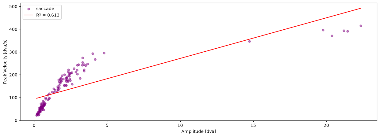
In this tutorial we will plot the saccadic main sequence of our data.
pm.plotting.main_sequence_plot(dataset.events[0])
(<Figure size 1500x500 with 1 Axes>,
 <Axes: xlabel='Amplitude [dva]', ylabel='Peak Velocity [dva/s]'>)
Saving and loading your dataframes#
If we want to save interim results, we can simply use the save() method like this:
dataset.save()
-
DatasetDefinitionDatasetDefinition
-
name:
'ToyDataset'
-
long_name:
'pymovements Toy Dataset'
-
'Example toy dataset. This dataset includes monocu...''Example toy dataset.\n\nThis dataset includes monocular eye tracking data from a single participant in a single\nsession. Eye movements are recorded at a sampling frequency of 1000 Hz using an EyeLink Portable\nDuo video-based eye tracker and are provided as pixel coordinates.\n\nThe participant is instructed to read 4 texts with 5 screens each.\n'
-
ExperimentExperiment
-
EyeTrackerEyeTracker
-
left:
None
-
model:
None
-
mount:
None
-
right:
None
-
sampling_rate:
1000
-
vendor:
None
-
version:
None
-
left:
-
ScreenScreen
-
distance_cm:
68
-
height_cm:
30.2
-
height_px:
1024
-
origin:
'upper left'
-
tuple (2 items)
- 1280
- 1024
-
tuple (2 items)
- 38
- 30.2
-
width_cm:
38
-
width_px:
1280
-
x_max_dva:
15.599386487782953
-
x_min_dva:
-15.599386487782953
-
y_max_dva:
12.508044410882546
-
y_min_dva:
-12.508044410882546
-
distance_cm:
-
-
list (1 items)
-
ResourceDefinition
-
content:
'gaze'
-
filename:
'pymovements-toy-dataset.zip'
-
filename_pattern:
'trial_{text_id:d}_{page_id:d}.csv'
-
dict (2 items)
-
text_id:
<class 'int'>
-
page_id:
<class 'int'>
-
text_id:
-
load_function:
None
-
dict (4 items)
-
time_column:
'timestamp'
-
time_unit:
'ms'
- (2 more)
-
time_column:
-
md5:
'256901852c1c07581d375eef705855d6'
-
mirrors:
None
-
WebSourceWebSource(url='https://github.com/pymovements/pymovements-toy-dataset/archive/refs/heads/main.zip', filename='pymovements-toy-dataset.zip', md5='256901852c1c07581d375eef705855d6', mirrors=None)
-
'https://github.com/pymovements/pymovements-toy-dat...''https://github.com/pymovements/pymovements-toy-dataset/archive/refs/heads/main.zip'
-
content:
-
ResourceDefinition
-
name:
-
tuple (1 items)
-
Events
-
DataFrame (7 columns, 264 rows)shape: (264, 7)
name onset offset duration dispersion amplitude peak_velocity str i64 i64 i64 f64 f64 f64 "fixation" 1988145 1988322 177 0.154958 0.110074 16.24151 "fixation" 1988351 1988546 195 0.291833 0.206397 18.88542 "fixation" 1988592 1988736 144 0.296297 0.209546 17.690373 "fixation" 1988788 1989012 224 0.271854 0.192719 19.130211 "fixation" 1989044 1989170 126 0.349 0.304362 18.616167 … … … … … … … "fixation_ivt" 2003929 2004090 161 2.814851 2.527788 212.117446 "fixation_ivt" 2004091 2004363 272 2.819008 2.518967 244.333244 "fixation_ivt" 2004364 2004883 519 2.768099 2.46208 194.527643 "fixation_ivt" 2004885 2005116 231 2.805674 2.507902 203.067333 "fixation_ivt" 2005117 2005298 181 2.744494 2.578767 329.741947 -
trial_columns:
None
-
-
Events
-
dict (1 items)
-
DataFrame (3 columns, 1 rows)shape: (1, 3)
text_id page_id filepath i64 i64 str 0 1 "pymovements-toy-dataset-main/d…
-
-
list (1 items)
-
Gaze
-
DataFrame (7 columns, 17223 rows)shape: (17_223, 7)
time stimuli_x stimuli_y pixel position velocity acceleration i64 f64 f64 list[f64] list[f64] list[f64] list[f64] 1988145 -1.0 -1.0 [206.8, 152.4] [-10.697598, -8.852399] [1.207641, -3.119165] [690.085837, -1501.799767] 1988146 -1.0 -1.0 [206.9, 152.1] [-10.695183, -8.859678] [1.20764, -4.072198] [0.001831, -866.371365] 1988147 -1.0 -1.0 [207.0, 151.8] [-10.692768, -8.866956] [1.035119, -4.765267] [-575.06741, -57.655244] 1988148 -1.0 -1.0 [207.1, 151.7] [-10.690352, -8.869381] [1.207654, -4.245382] [-230.013049, 1328.57081] 1988149 -1.0 -1.0 [207.0, 151.5] [-10.692768, -8.874233] [1.552735, -2.339263] [690.12611, 2021.586565] … … … … … … … 2005363 -1.0 -1.0 [361.0, 415.4] [-6.932438, -2.386672] [-62.062479, -20.465552] [-1099.087619, 1477.17518] 2005364 -1.0 -1.0 [358.0, 414.5] [-7.006376, -2.408998] [-61.343786, -18.073031] [1834.348384, 2599.156806] 2005365 -1.0 -1.0 [355.8, 413.8] [-7.060582, -2.426362] [-53.501231, -14.617634] [9396.15507, 4547.960553] 2005366 -1.0 -1.0 [353.1, 413.2] [-7.12709, -2.441245] [-41.879965, -10.276475] [16194.183852, 5079.286997] 2005367 -1.0 -1.0 [351.2, 412.9] [-7.173881, -2.448686] [-27.710881, -6.112645] [16598.914618, 4193.246498] -
EventsEvents
-
DataFrame (7 columns, 264 rows)shape: (264, 7)
name onset offset duration dispersion amplitude peak_velocity str i64 i64 i64 f64 f64 f64 "fixation" 1988145 1988322 177 0.154958 0.110074 16.24151 "fixation" 1988351 1988546 195 0.291833 0.206397 18.88542 "fixation" 1988592 1988736 144 0.296297 0.209546 17.690373 "fixation" 1988788 1989012 224 0.271854 0.192719 19.130211 "fixation" 1989044 1989170 126 0.349 0.304362 18.616167 … … … … … … … "fixation_ivt" 2003929 2004090 161 2.814851 2.527788 212.117446 "fixation_ivt" 2004091 2004363 272 2.819008 2.518967 244.333244 "fixation_ivt" 2004364 2004883 519 2.768099 2.46208 194.527643 "fixation_ivt" 2004885 2005116 231 2.805674 2.507902 203.067333 "fixation_ivt" 2005117 2005298 181 2.744494 2.578767 329.741947 -
trial_columns:
None
-
-
dict (2 items)
-
text_id:
0
-
page_id:
1
-
text_id:
-
messages:
None
-
trial_columns:
None
-
ExperimentExperiment
-
EyeTrackerEyeTracker
-
left:
None
-
model:
None
-
mount:
None
-
right:
None
-
sampling_rate:
1000
-
vendor:
None
-
version:
None
-
left:
-
ScreenScreen
-
distance_cm:
68
-
height_cm:
30.2
-
height_px:
1024
-
origin:
'upper left'
-
tuple (2 items)
- 1280
- 1024
-
tuple (2 items)
- 38
- 30.2
-
width_cm:
38
-
width_px:
1280
-
x_max_dva:
15.599386487782953
-
x_min_dva:
-15.599386487782953
-
y_max_dva:
12.508044410882546
-
y_min_dva:
-12.508044410882546
-
distance_cm:
-
-
-
Gaze
-
ParticipantsParticipants
-
DataFrame (1 columns, 0 rows)shape: (0, 1)
participant_id str -
dict (1 items)
-
dict (1 items)
-
Format:
'string'
-
Format:
-
-
-
path:
PosixPath('data/ToyDataset')
-
DatasetPathsDatasetPaths
-
dataset:
PosixPath('data/ToyDataset')
-
downloads:
PosixPath('data/ToyDataset/downloads')
-
events:
PosixPath('data/ToyDataset/events')
-
precomputed_events:
PosixPath('data/ToyDataset/precomputed_events')
-
precomputed_reading_measures:
PosixPath('data/ToyDataset/precomputed_reading_measures')
-
preprocessed:
PosixPath('data/ToyDataset/preprocessed')
-
raw:
PosixPath('data/ToyDataset/raw')
-
root:
PosixPath('data/ToyDataset')
-
stimuli:
PosixPath('data/ToyDataset/stimuli')
-
dataset:
-
precomputed_events:
list (0 items)
-
precomputed_reading_measures:
list (0 items)
-
stimuli:
list (0 items)
Let’s test this out by initializing a new PublicDataset object in the same directory and loading in the preprocessed gaze and event data.
This time we don’t need to download anything.
preprocessed_dataset = pm.Dataset('ToyDataset', path='data/ToyDataset')

dataset.load(events=True, preprocessed=True, subset=subset)

display(dataset.gaze[0])
display(dataset.events[0])
-
DataFrame (7 columns, 17223 rows)shape: (17_223, 7)
time stimuli_x stimuli_y pixel position velocity acceleration i64 f64 f64 list[f64] list[f64] list[f64] list[f64] 1988145 -1.0 -1.0 [206.8, 152.4] [-10.697598, -8.852399] [1.207641, -3.119165] [690.085837, -1501.799767] 1988146 -1.0 -1.0 [206.9, 152.1] [-10.695183, -8.859678] [1.20764, -4.072198] [0.001831, -866.371365] 1988147 -1.0 -1.0 [207.0, 151.8] [-10.692768, -8.866956] [1.035119, -4.765267] [-575.06741, -57.655244] 1988148 -1.0 -1.0 [207.1, 151.7] [-10.690352, -8.869381] [1.207654, -4.245382] [-230.013049, 1328.57081] 1988149 -1.0 -1.0 [207.0, 151.5] [-10.692768, -8.874233] [1.552735, -2.339263] [690.12611, 2021.586565] … … … … … … … 2005363 -1.0 -1.0 [361.0, 415.4] [-6.932438, -2.386672] [-62.062479, -20.465552] [-1099.087619, 1477.17518] 2005364 -1.0 -1.0 [358.0, 414.5] [-7.006376, -2.408998] [-61.343786, -18.073031] [1834.348384, 2599.156806] 2005365 -1.0 -1.0 [355.8, 413.8] [-7.060582, -2.426362] [-53.501231, -14.617634] [9396.15507, 4547.960553] 2005366 -1.0 -1.0 [353.1, 413.2] [-7.12709, -2.441245] [-41.879965, -10.276475] [16194.183852, 5079.286997] 2005367 -1.0 -1.0 [351.2, 412.9] [-7.173881, -2.448686] [-27.710881, -6.112645] [16598.914618, 4193.246498] -
EventsEvents
-
DataFrame (7 columns, 264 rows)shape: (264, 7)
name onset offset duration dispersion amplitude peak_velocity str i64 i64 i64 f64 f64 f64 "fixation" 1988145 1988322 177 0.154958 0.110074 16.24151 "fixation" 1988351 1988546 195 0.291833 0.206397 18.88542 "fixation" 1988592 1988736 144 0.296297 0.209546 17.690373 "fixation" 1988788 1989012 224 0.271854 0.192719 19.130211 "fixation" 1989044 1989170 126 0.349 0.304362 18.616167 … … … … … … … "fixation_ivt" 2003929 2004090 161 2.814851 2.527788 212.117446 "fixation_ivt" 2004091 2004363 272 2.819008 2.518967 244.333244 "fixation_ivt" 2004364 2004883 519 2.768099 2.46208 194.527643 "fixation_ivt" 2004885 2005116 231 2.805674 2.507902 203.067333 "fixation_ivt" 2005117 2005298 181 2.744494 2.578767 329.741947 -
trial_columns:
None
-
-
dict (2 items)
-
text_id:
0
-
page_id:
1
-
text_id:
-
messages:
None
-
trial_columns:
None
-
ExperimentExperiment
-
EyeTrackerEyeTracker
-
left:
None
-
model:
None
-
mount:
None
-
right:
None
-
sampling_rate:
1000
-
vendor:
None
-
version:
None
-
left:
-
ScreenScreen
-
distance_cm:
68
-
height_cm:
30.2
-
height_px:
1024
-
origin:
'upper left'
-
tuple (2 items)
- 1280
- 1024
-
tuple (2 items)
- 38
- 30.2
-
width_cm:
38
-
width_px:
1280
-
x_max_dva:
15.599386487782953
-
x_min_dva:
-15.599386487782953
-
y_max_dva:
12.508044410882546
-
y_min_dva:
-12.508044410882546
-
distance_cm:
-
-
DataFrame (7 columns, 264 rows)shape: (264, 7)
name onset offset duration dispersion amplitude peak_velocity str i64 i64 i64 f64 f64 f64 "fixation" 1988145 1988322 177 0.154958 0.110074 16.24151 "fixation" 1988351 1988546 195 0.291833 0.206397 18.88542 "fixation" 1988592 1988736 144 0.296297 0.209546 17.690373 "fixation" 1988788 1989012 224 0.271854 0.192719 19.130211 "fixation" 1989044 1989170 126 0.349 0.304362 18.616167 … … … … … … … "fixation_ivt" 2003929 2004090 161 2.814851 2.527788 212.117446 "fixation_ivt" 2004091 2004363 272 2.819008 2.518967 244.333244 "fixation_ivt" 2004364 2004883 519 2.768099 2.46208 194.527643 "fixation_ivt" 2004885 2005116 231 2.805674 2.507902 203.067333 "fixation_ivt" 2005117 2005298 181 2.744494 2.578767 329.741947 -
trial_columns:
None