Plot saccadic main sequence

In this notebook we show how you can load a dataset, compute all the necessary properties and the plot the main sequence.

What you will learn in this tutorial:

• how to prepare your data to plot the saccadic main sequence

• how to create a main sequence plot of your saccade events

Loading and preprocessing your data

import pymovements as pm
from pymovements.events import microsaccades
from pymovements.plotting import main_sequence_plot

/home/docs/checkouts/readthedocs.org/user_builds/pymovements/envs/v0.7.0/lib/python3.9/site-packages/tqdm/auto.py:21: TqdmWarning: IProgress not found. Please update jupyter and ipywidgets. See https://ipywidgets.readthedocs.io/en/stable/user_install.html
  from .autonotebook import tqdm as notebook_tqdm

First, you have to define your dataset. You can already download and extract all the files.

dataset = pm.datasets.toy_dataset.ToyDataset(
    root='data/', download=True, extract=True, remove_finished=True)
dataset.load()

Downloading http://github.com/aeye-lab/pymovements-toy-dataset/zipball/6cb5d663317bf418cec0c9abe1dde5085a8a8ebd/ to data/ToyDataset/downloads/pymovements-toy-dataset.zip

pymovements-toy-dataset.zip: 100%|██████████| 3.06M/3.06M [00:00<00:00, 24.6MB/s]
100%|██████████| 20/20 [00:00<00:00, 199.85it/s]

Now, you have to convert the raw x and y coordinates in pixels to degrees in visual angle.

dataset.pix2deg()

100%|██████████| 20/20 [00:00<00:00, 739.06it/s]

Next we can convert these positions into velocitites.

dataset.pos2vel()

100%|██████████| 20/20 [00:00<00:00, 675.32it/s]

Let’s check if we now have all our expected columns:

dataset.gaze[0].frame.head()

shape: (5, 9)

text_id	page_id	time	x_right_pix	y_right_pix	x_right_pos	y_right_pos	x_right_vel	y_right_vel
i64	i64	f64	f64	f64	f64	f64	f64	f64
0	1	1.988145e6	206.8	152.4	-10.697598	-8.852399	1.207626	-3.639106
0	1	1.988146e6	206.9	152.1	-10.695183	-8.859678	2.415272	-7.278067
0	1	1.988147e6	207.0	151.8	-10.692768	-8.866956	1.610194	-5.256267
0	1	1.988148e6	207.1	151.7	-10.690352	-8.869381	0.402548	-4.447465
0	1	1.988149e6	207.0	151.5	-10.692768	-8.874233	0.402561	-3.234462

Detecting your events and compute properties

In the next step we have to detect our saccades and compute the event properties amplitude and peak_velocity.

We can run the microsaccade detection algorithm with its default parameters:

dataset.detect_events(microsaccades)

20it [00:00, 65.50it/s]

Next we compute the event properties ‘amplitude’ and ‘peak velocity’ for the detected saccades.

dataset.compute_event_properties(['amplitude', 'peak_velocity'])

20it [00:13,  1.49it/s]

Let’s verify that we have detected some saccades and have the desired columns available.

dataset.events[0].frame.head()

shape: (5, 8)

text_id	page_id	name	onset	offset	duration	amplitude	peak_velocity
i64	i64	str	i64	i64	i64	f64	f64
0	1	"saccade"	1988323	1988337	14	3.400319	223.354404
0	1	"saccade"	1988342	1988350	8	0.337405	43.903782
0	1	"saccade"	1988547	1988567	20	1.823525	176.116206
0	1	"saccade"	1988571	1988582	11	0.983307	100.904927
0	1	"saccade"	1988737	1988760	23	21.40854	393.897938

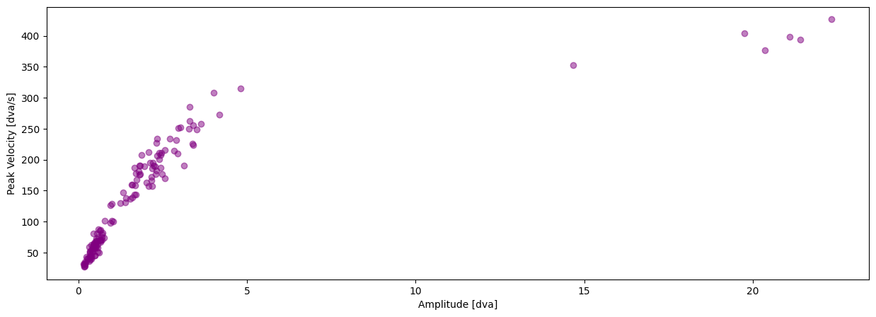
Plot the main sequence

Now we just pass the event dataframe to the plotting function:

# only showing the first three event dataframes here.
for event_df in dataset.events[:3]:
    print(
        f'Showing main sequence plot for '
        f'text {event_df[0, "text_id"]}, '
        f'page {event_df[0, "page_id"]}:')
    main_sequence_plot(event_df)

Showing main sequence plot for text 0, page 1:

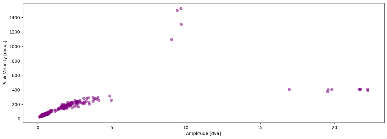
Showing main sequence plot for text 0, page 2:

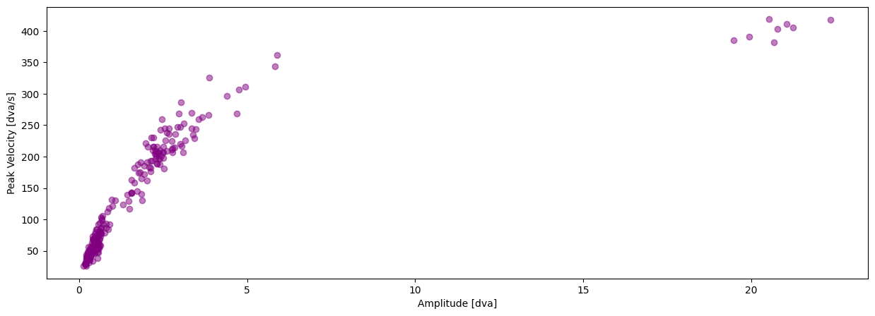
Showing main sequence plot for text 0, page 3:

What you have learned in this tutorial:

• how to prepare your data to plot a main sequence

• how to create a main sequence plot by using main_sequence_plot