Plot saccadic main sequence#
In this notebook we show how you can load a dataset, compute all the necessary properties and the plot the main sequence.
What you will learn in this tutorial:#
how to prepare your data to plot the saccadic main sequence
how to create a main sequence plot of your saccade events and style it to your liking
Loading and preprocessing your data#
We import pymovements as the alias pm for convenience.
[1]:
import pymovements as pm
/home/docs/checkouts/readthedocs.org/user_builds/pymovements/envs/v0.21.2/lib/python3.9/site-packages/tqdm/auto.py:21: TqdmWarning: IProgress not found. Please update jupyter and ipywidgets. See https://ipywidgets.readthedocs.io/en/stable/user_install.html
  from .autonotebook import tqdm as notebook_tqdm
Let’s start by downloading our ToyDataset and loading in its data:
[2]:
dataset = pm.Dataset('ToyDataset', path='data/ToyDataset')
dataset.download()
dataset.load()
INFO:pymovements.dataset.dataset_download:You are downloading the pymovements Toy Dataset. Please be aware that pymovements does not
host or distribute any dataset resources and only provides a convenient interface to
download the public dataset resources that were published by their respective authors.

Please cite the referenced publication if you intend to use the dataset in your research.
Using already downloaded and verified file: data/ToyDataset/downloads/pymovements-toy-dataset.zip
Extracting pymovements-toy-dataset.zip to data/ToyDataset/raw
100%|██████████| 23/23 [00:00<00:00, 200.48it/s]
100%|██████████| 20/20 [00:00<00:00, 26.53it/s]
[2]:
<pymovements.dataset.dataset.Dataset at 0x7a019c1f3ca0>
Now, you have to convert the raw x and y coordinates in pixels to degrees in visual angle.
[3]:
dataset.pix2deg()
100%|██████████| 20/20 [00:01<00:00, 13.91it/s]
[3]:
<pymovements.dataset.dataset.Dataset at 0x7a019c1f3ca0>
Next we can convert these positions into velocitites.
[4]:
dataset.pos2vel()
100%|██████████| 20/20 [00:00<00:00, 29.82it/s]
[4]:
<pymovements.dataset.dataset.Dataset at 0x7a019c1f3ca0>
Let’s check if we now have all our expected columns:
[5]:
dataset.gaze[0]
[5]:
Experiment(screen=Screen(width_px=1280, height_px=1024, width_cm=38, height_cm=30.2, distance_cm=68, origin='upper left'), eyetracker=EyeTracker(sampling_rate=1000, left=None, right=None, model=None, version=None, vendor=None, mount=None))
shape: (17_223, 8)
┌─────────┬───────────┬───────────┬─────────┬─────────┬───────────┬────────────────┬───────────────┐
│ time    ┆ stimuli_x ┆ stimuli_y ┆ text_id ┆ page_id ┆ pixel     ┆ position       ┆ velocity      │
│ ---     ┆ ---       ┆ ---       ┆ ---     ┆ ---     ┆ ---       ┆ ---            ┆ ---           │
│ i64     ┆ f64       ┆ f64       ┆ i64     ┆ i64     ┆ list[f64] ┆ list[f64]      ┆ list[f64]     │
╞═════════╪═══════════╪═══════════╪═════════╪═════════╪═══════════╪════════════════╪═══════════════╡
│ 1988145 ┆ -1.0      ┆ -1.0      ┆ 0       ┆ 1       ┆ [206.8,   ┆ [-10.697598,   ┆ [null, null]  │
│         ┆           ┆           ┆         ┆         ┆ 152.4]    ┆ -8.852399]     ┆               │
│ 1988146 ┆ -1.0      ┆ -1.0      ┆ 0       ┆ 1       ┆ [206.9,   ┆ [-10.695183,   ┆ [null, null]  │
│         ┆           ┆           ┆         ┆         ┆ 152.1]    ┆ -8.859678]     ┆               │
│ 1988147 ┆ -1.0      ┆ -1.0      ┆ 0       ┆ 1       ┆ [207.0,   ┆ [-10.692768,   ┆ [1.610194,    │
│         ┆           ┆           ┆         ┆         ┆ 151.8]    ┆ -8.866956]     ┆ -5.256267]    │
│ 1988148 ┆ -1.0      ┆ -1.0      ┆ 0       ┆ 1       ┆ [207.1,   ┆ [-10.690352,   ┆ [0.402548,    │
│         ┆           ┆           ┆         ┆         ┆ 151.7]    ┆ -8.869381]     ┆ -4.447465]    │
│ 1988149 ┆ -1.0      ┆ -1.0      ┆ 0       ┆ 1       ┆ [207.0,   ┆ [-10.692768,   ┆ [0.402561,    │
│         ┆           ┆           ┆         ┆         ┆ 151.5]    ┆ -8.874233]     ┆ -3.234462]    │
│ …       ┆ …         ┆ …         ┆ …       ┆ …       ┆ …         ┆ …              ┆ …             │
│ 2005363 ┆ -1.0      ┆ -1.0      ┆ 0       ┆ 1       ┆ [361.0,   ┆ [-6.932438,    ┆ [-63.266374,  │
│         ┆           ┆           ┆         ┆         ┆ 415.4]    ┆ -2.386672]     ┆ -21.085616]   │
│ 2005364 ┆ -1.0      ┆ -1.0      ┆ 0       ┆ 1       ┆ [358.0,   ┆ [-7.006376,    ┆ [-63.249652,  │
│         ┆           ┆           ┆         ┆         ┆ 414.5]    ┆ -2.408998]     ┆ -19.431326]   │
│ 2005365 ┆ -1.0      ┆ -1.0      ┆ 0       ┆ 1       ┆ [355.8,   ┆ [-7.060582,    ┆ [-60.359624,  │
│         ┆           ┆           ┆         ┆         ┆ 413.8]    ┆ -2.426362]     ┆ -15.710061]   │
│ 2005366 ┆ -1.0      ┆ -1.0      ┆ 0       ┆ 1       ┆ [353.1,   ┆ [-7.12709,     ┆ [null, null]  │
│         ┆           ┆           ┆         ┆         ┆ 413.2]    ┆ -2.441245]     ┆               │
│ 2005367 ┆ -1.0      ┆ -1.0      ┆ 0       ┆ 1       ┆ [351.2,   ┆ [-7.173881,    ┆ [null, null]  │
│         ┆           ┆           ┆         ┆         ┆ 412.9]    ┆ -2.448686]     ┆               │
└─────────┴───────────┴───────────┴─────────┴─────────┴───────────┴────────────────┴───────────────┘
Detecting your events and compute properties#
In the next step we have to detect our saccades and compute the event properties amplitude and peak_velocity.
We can run the microsaccade detection algorithm with its default parameters:
[6]:
dataset.detect_events('microsaccades')
20it [00:00, 42.51it/s]
[6]:
<pymovements.dataset.dataset.Dataset at 0x7a019c1f3ca0>
Next we compute the event properties ‘amplitude’ and ‘peak velocity’ for the detected saccades.
[7]:
dataset.compute_event_properties(['amplitude', 'peak_velocity'])
100%|██████████| 20/20 [00:05<00:00, 3.93it/s]
[7]:
<pymovements.dataset.dataset.Dataset at 0x7a019c1f3ca0>
Let’s verify that we have detected some saccades and have the desired columns available.
[8]:
dataset.events[0]
[8]:
shape: (142, 8)
┌─────────┬─────────┬─────────┬─────────┬─────────┬──────────┬───────────┬───────────────┐
│ text_id ┆ page_id ┆ name    ┆ onset   ┆ offset  ┆ duration ┆ amplitude ┆ peak_velocity │
│ ---     ┆ ---     ┆ ---     ┆ ---     ┆ ---     ┆ ---      ┆ ---       ┆ ---           │
│ i64     ┆ i64     ┆ str     ┆ i64     ┆ i64     ┆ i64      ┆ f64       ┆ f64           │
╞═════════╪═════════╪═════════╪═════════╪═════════╪══════════╪═══════════╪═══════════════╡
│ 0       ┆ 1       ┆ saccade ┆ 1988323 ┆ 1988337 ┆ 14       ┆ 1.236741  ┆ 129.856451    │
│ 0       ┆ 1       ┆ saccade ┆ 1988342 ┆ 1988350 ┆ 8        ┆ 0.330748  ┆ 50.527286     │
│ 0       ┆ 1       ┆ saccade ┆ 1988547 ┆ 1988567 ┆ 20       ┆ 2.391184  ┆ 200.144558    │
│ 0       ┆ 1       ┆ saccade ┆ 1988571 ┆ 1988582 ┆ 11       ┆ 0.476811  ┆ 56.048003     │
│ 0       ┆ 1       ┆ saccade ┆ 1988737 ┆ 1988760 ┆ 23       ┆ 3.285115  ┆ 249.67823     │
│ …       ┆ …       ┆ …       ┆ …       ┆ …       ┆ …        ┆ …         ┆ …             │
│ 0       ┆ 1       ┆ saccade ┆ 2005110 ┆ 2005126 ┆ 16       ┆ 1.405354  ┆ 137.917594    │
│ 0       ┆ 1       ┆ saccade ┆ 2005128 ┆ 2005138 ┆ 10       ┆ 0.44098   ┆ 61.197926     │
│ 0       ┆ 1       ┆ saccade ┆ 2005288 ┆ 2005345 ┆ 57       ┆ 14.682541 ┆ 352.550667    │
│ 0       ┆ 1       ┆ saccade ┆ 2005347 ┆ 2005356 ┆ 9        ┆ 0.629861  ┆ 85.484987     │
│ 0       ┆ 1       ┆ saccade ┆ 2005359 ┆ 2005365 ┆ 6        ┆ 0.368268  ┆ 66.68761      │
└─────────┴─────────┴─────────┴─────────┴─────────┴──────────┴───────────┴───────────────┘
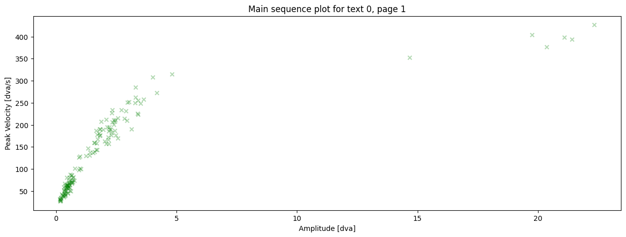
Plot the main sequence#
Now we just pass the event dataframe to the plotting function:
[9]:
# only showing the first three event dataframes here.
# note that you can adjust the styling of the plot, e.g. setting a low
# alpha value allows you to see overlapping data points
for event_df in dataset.events[:3]:
    pm.plotting.main_sequence_plot(
        event_df,
        title='Main sequence plot for '
        f'text {event_df[0, "text_id"]}, '
        f'page {event_df[0, "page_id"]}',
        alpha=0.3,
        color='green',
        marker='x',
        marker_size=30,
    )
What you have learned in this tutorial:#
how to prepare your data to plot a main sequence
how to create a main sequence plot by using
main_sequence_plot