Plot saccadic main sequence#
In this notebook we show how you can load a dataset, compute all the necessary properties and the plot the main sequence.
What you will learn in this tutorial:#
how to prepare your data to plot the saccadic main sequence
how to create a main sequence plot of your saccade events and style it to your liking
Loading and preprocessing your data#
We import pymovements as the alias pm for convenience.
[1]:
import pymovements as pm
/home/docs/checkouts/readthedocs.org/user_builds/pymovements/envs/v0.19.0/lib/python3.9/site-packages/tqdm/auto.py:21: TqdmWarning: IProgress not found. Please update jupyter and ipywidgets. See https://ipywidgets.readthedocs.io/en/stable/user_install.html
  from .autonotebook import tqdm as notebook_tqdm
Let’s start by downloading our ToyDataset and loading in its data:
[2]:
dataset = pm.Dataset('ToyDataset', path='data/ToyDataset')
dataset.download()
dataset.load()
Using already downloaded and verified file: data/ToyDataset/downloads/pymovements-toy-dataset.zip
Extracting pymovements-toy-dataset.zip to data/ToyDataset/raw
100%|██████████| 20/20 [00:00<00:00, 38.87it/s]
[2]:
<pymovements.dataset.dataset.Dataset at 0x7f988c232430>
Now, you have to convert the raw x and y coordinates in pixels to degrees in visual angle.
[3]:
dataset.pix2deg()
100%|██████████| 20/20 [00:01<00:00, 18.21it/s]
[3]:
<pymovements.dataset.dataset.Dataset at 0x7f988c232430>
Next we can convert these positions into velocitites.
[4]:
dataset.pos2vel()
100%|██████████| 20/20 [00:00<00:00, 36.79it/s]
[4]:
<pymovements.dataset.dataset.Dataset at 0x7f988c232430>
Let’s check if we now have all our expected columns:
[5]:
dataset.gaze[0]
[5]:
Experiment(sampling_rate=1000, screen=Screen(width_px=1280, height_px=1024, width_cm=38, height_cm=30.20, distance_cm=68, origin=upper left), eyetracker=None)
shape: (17_223, 8)
┌─────────┬───────────┬───────────┬─────────┬─────────┬───────────┬────────────────┬───────────────┐
│ time    ┆ stimuli_x ┆ stimuli_y ┆ text_id ┆ page_id ┆ pixel     ┆ position       ┆ velocity      │
│ ---     ┆ ---       ┆ ---       ┆ ---     ┆ ---     ┆ ---       ┆ ---            ┆ ---           │
│ i64     ┆ f64       ┆ f64       ┆ i64     ┆ i64     ┆ list[f64] ┆ list[f64]      ┆ list[f64]     │
╞═════════╪═══════════╪═══════════╪═════════╪═════════╪═══════════╪════════════════╪═══════════════╡
│ 1988145 ┆ -1.0      ┆ -1.0      ┆ 0       ┆ 1       ┆ [206.8,   ┆ [-10.697598,   ┆ [null, null]  │
│         ┆           ┆           ┆         ┆         ┆ 152.4]    ┆ -8.852399]     ┆               │
│ 1988146 ┆ -1.0      ┆ -1.0      ┆ 0       ┆ 1       ┆ [206.9,   ┆ [-10.695183,   ┆ [null, null]  │
│         ┆           ┆           ┆         ┆         ┆ 152.1]    ┆ -8.859678]     ┆               │
│ 1988147 ┆ -1.0      ┆ -1.0      ┆ 0       ┆ 1       ┆ [207.0,   ┆ [-10.692768,   ┆ [1.610194,    │
│         ┆           ┆           ┆         ┆         ┆ 151.8]    ┆ -8.866956]     ┆ -5.256267]    │
│ 1988148 ┆ -1.0      ┆ -1.0      ┆ 0       ┆ 1       ┆ [207.1,   ┆ [-10.690352,   ┆ [0.402548,    │
│         ┆           ┆           ┆         ┆         ┆ 151.7]    ┆ -8.869381]     ┆ -4.447465]    │
│ 1988149 ┆ -1.0      ┆ -1.0      ┆ 0       ┆ 1       ┆ [207.0,   ┆ [-10.692768,   ┆ [0.402561,    │
│         ┆           ┆           ┆         ┆         ┆ 151.5]    ┆ -8.874233]     ┆ -3.234462]    │
│ …       ┆ …         ┆ …         ┆ …       ┆ …       ┆ …         ┆ …              ┆ …             │
│ 2005363 ┆ -1.0      ┆ -1.0      ┆ 0       ┆ 1       ┆ [361.0,   ┆ [-6.932438,    ┆ [-63.266374,  │
│         ┆           ┆           ┆         ┆         ┆ 415.4]    ┆ -2.386672]     ┆ -21.085616]   │
│ 2005364 ┆ -1.0      ┆ -1.0      ┆ 0       ┆ 1       ┆ [358.0,   ┆ [-7.006376,    ┆ [-63.249652,  │
│         ┆           ┆           ┆         ┆         ┆ 414.5]    ┆ -2.408998]     ┆ -19.431326]   │
│ 2005365 ┆ -1.0      ┆ -1.0      ┆ 0       ┆ 1       ┆ [355.8,   ┆ [-7.060582,    ┆ [-60.359624,  │
│         ┆           ┆           ┆         ┆         ┆ 413.8]    ┆ -2.426362]     ┆ -15.710061]   │
│ 2005366 ┆ -1.0      ┆ -1.0      ┆ 0       ┆ 1       ┆ [353.1,   ┆ [-7.12709,     ┆ [null, null]  │
│         ┆           ┆           ┆         ┆         ┆ 413.2]    ┆ -2.441245]     ┆               │
│ 2005367 ┆ -1.0      ┆ -1.0      ┆ 0       ┆ 1       ┆ [351.2,   ┆ [-7.173881,    ┆ [null, null]  │
│         ┆           ┆           ┆         ┆         ┆ 412.9]    ┆ -2.448686]     ┆               │
└─────────┴───────────┴───────────┴─────────┴─────────┴───────────┴────────────────┴───────────────┘
Detecting your events and compute properties#
In the next step we have to detect our saccades and compute the event properties amplitude and peak_velocity.
We can run the microsaccade detection algorithm with its default parameters:
[6]:
dataset.detect_events('microsaccades')
20it [00:00, 36.94it/s]
[6]:
<pymovements.dataset.dataset.Dataset at 0x7f988c232430>
Next we compute the event properties ‘amplitude’ and ‘peak velocity’ for the detected saccades.
[7]:
dataset.compute_event_properties(['amplitude', 'peak_velocity'])
20it [00:03, 6.19it/s]
[7]:
<pymovements.dataset.dataset.Dataset at 0x7f988c232430>
Let’s verify that we have detected some saccades and have the desired columns available.
[8]:
dataset.events[0]
[8]:
shape: (142, 8)
┌─────────┬─────────┬─────────┬─────────┬─────────┬──────────┬───────────┬───────────────┐
│ text_id ┆ page_id ┆ name    ┆ onset   ┆ offset  ┆ duration ┆ amplitude ┆ peak_velocity │
│ ---     ┆ ---     ┆ ---     ┆ ---     ┆ ---     ┆ ---      ┆ ---       ┆ ---           │
│ i64     ┆ i64     ┆ str     ┆ i64     ┆ i64     ┆ i64      ┆ f64       ┆ f64           │
╞═════════╪═════════╪═════════╪═════════╪═════════╪══════════╪═══════════╪═══════════════╡
│ 0       ┆ 1       ┆ saccade ┆ 1988323 ┆ 1988337 ┆ 14       ┆ 1.236741  ┆ 129.856451    │
│ 0       ┆ 1       ┆ saccade ┆ 1988342 ┆ 1988350 ┆ 8        ┆ 0.330748  ┆ 50.527286     │
│ 0       ┆ 1       ┆ saccade ┆ 1988547 ┆ 1988567 ┆ 20       ┆ 2.391184  ┆ 200.144558    │
│ 0       ┆ 1       ┆ saccade ┆ 1988571 ┆ 1988582 ┆ 11       ┆ 0.476811  ┆ 56.048003     │
│ 0       ┆ 1       ┆ saccade ┆ 1988737 ┆ 1988760 ┆ 23       ┆ 3.285115  ┆ 249.67823     │
│ …       ┆ …       ┆ …       ┆ …       ┆ …       ┆ …        ┆ …         ┆ …             │
│ 0       ┆ 1       ┆ saccade ┆ 2005110 ┆ 2005126 ┆ 16       ┆ 1.405354  ┆ 137.917594    │
│ 0       ┆ 1       ┆ saccade ┆ 2005128 ┆ 2005138 ┆ 10       ┆ 0.44098   ┆ 61.197926     │
│ 0       ┆ 1       ┆ saccade ┆ 2005288 ┆ 2005345 ┆ 57       ┆ 14.682541 ┆ 352.550667    │
│ 0       ┆ 1       ┆ saccade ┆ 2005347 ┆ 2005356 ┆ 9        ┆ 0.629861  ┆ 85.484987     │
│ 0       ┆ 1       ┆ saccade ┆ 2005359 ┆ 2005365 ┆ 6        ┆ 0.368268  ┆ 66.68761      │
└─────────┴─────────┴─────────┴─────────┴─────────┴──────────┴───────────┴───────────────┘
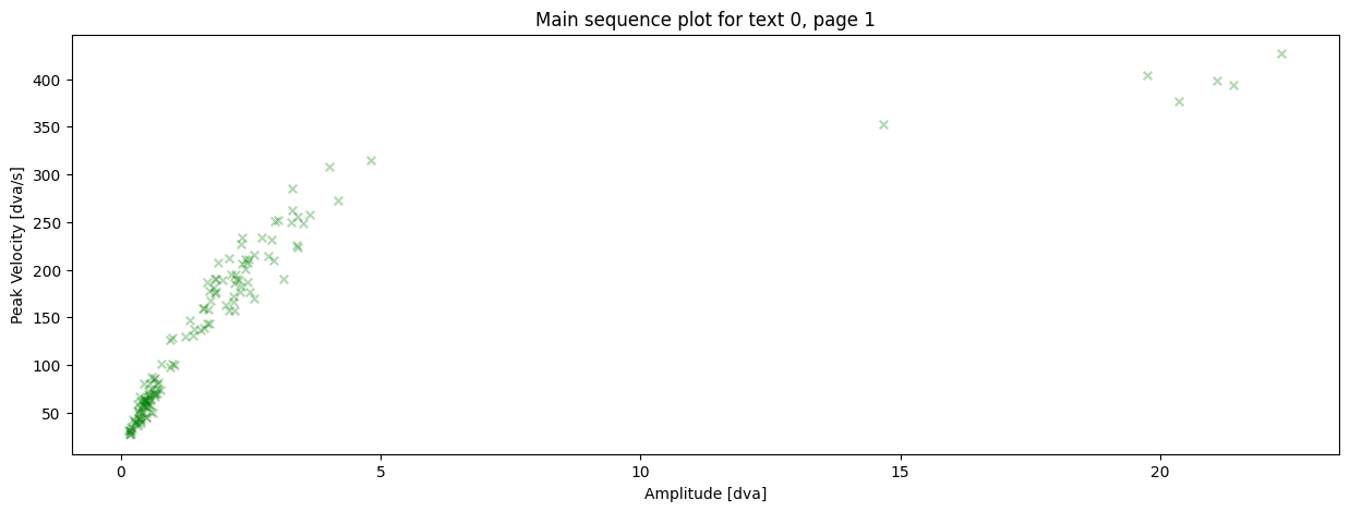
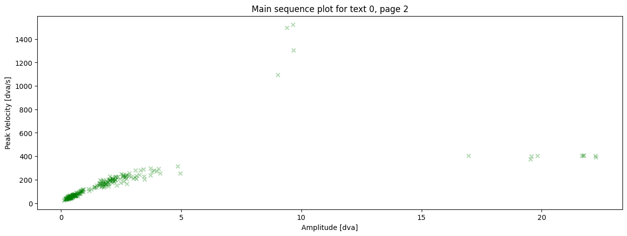
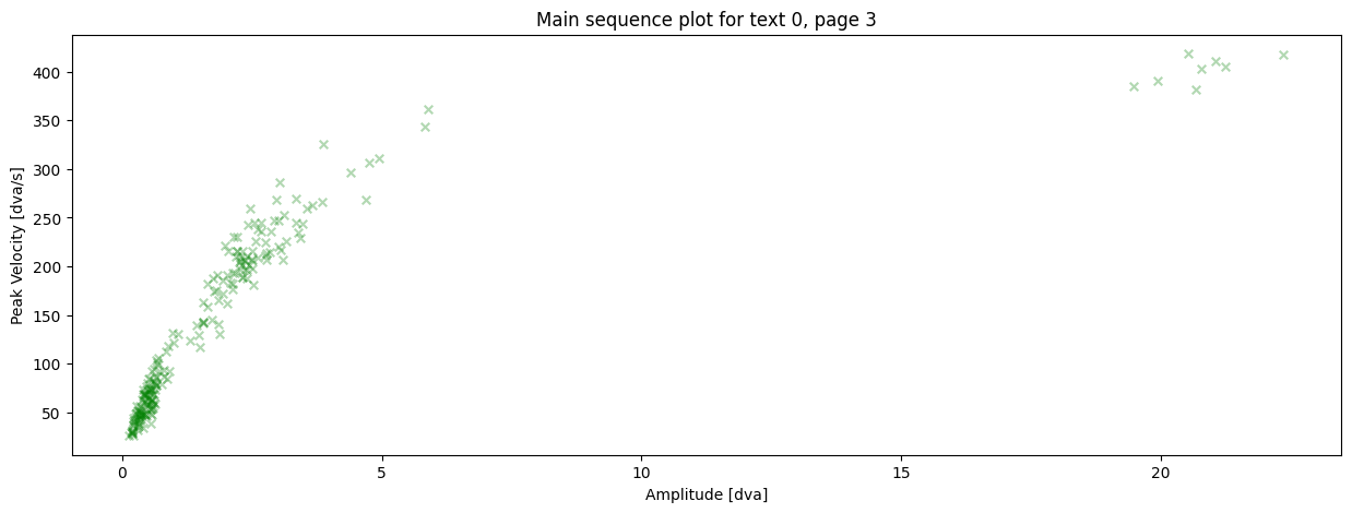
Plot the main sequence#
Now we just pass the event dataframe to the plotting function:
[9]:
# only showing the first three event dataframes here.
# note that you can adjust the styling of the plot, e.g. setting a low
# alpha value allows you to see overlapping data points
for event_df in dataset.events[:3]:
    pm.plotting.main_sequence_plot(
        event_df,
        title='Main sequence plot for '
        f'text {event_df[0, "text_id"]}, '
        f'page {event_df[0, "page_id"]}',
        alpha=0.3,
        color='green',
        marker='x',
        marker_size=30,
    )
What you have learned in this tutorial:#
how to prepare your data to plot a main sequence
how to create a main sequence plot by using
main_sequence_plot