pymovements in 10 minutes#
What you will learn in this tutorial:#
how to download one of the publicly available datasets
how to load a subset of the data into your memory
how to transform pixel coordinates into degrees of visual angle
how to transform positional data into velocity data
how to detect fixations by using the I-DT algorithm
how to detect saccades by using the microsaccades algorithm
how to compute additional event properties for your analysis
how to save your preprocessed data
how to plot the main saccadic sequence from your data
Downloading one of the public datasets#
We import pymovements as the alias pm for convenience.
[1]:
import polars as pl

import pymovements as pm
/home/docs/checkouts/readthedocs.org/user_builds/pymovements/envs/v0.10.0/lib/python3.9/site-packages/tqdm/auto.py:21: TqdmWarning: IProgress not found. Please update jupyter and ipywidgets. See https://ipywidgets.readthedocs.io/en/stable/user_install.html
  from .autonotebook import tqdm as notebook_tqdm
pymovements provides a library of publicly available datasets.
You can browse through the available dataset definitions here: Datasets
For this tutorial we will limit ourselves to the ToyDataset due to its minimal space requirements.
Other datasets can be downloaded by simply replacing ToyDataset with one of the other available datasets.
We can initialize and download by passing the desired dataset name as a string argument.
Additionally we need the root directory path of your data.
[2]:
dataset = pm.Dataset('ToyDataset', path='data/ToyDataset')
dataset.download()
Downloading http://github.com/aeye-lab/pymovements-toy-dataset/zipball/6cb5d663317bf418cec0c9abe1dde5085a8a8ebd/ to data/ToyDataset/downloads/pymovements-toy-dataset.zip
pymovements-toy-dataset.zip: 100%|██████████| 3.06M/3.06M [00:00<00:00, 22.8MB/s]
[2]:
<pymovements.dataset.dataset.Dataset at 0x7fa3e6ab57c0>
Our downloaded dataset will be placed in new a directory with the name of the dataset:
[3]:
dataset.path
[3]:
PosixPath('data/ToyDataset')
Archive files are automatically extracted into the path specified by Dataset.paths.raw:
[4]:
dataset.paths.raw
[4]:
PosixPath('data/ToyDataset/raw')
Loading in your data into memory#
Next we load our dataset into memory to be able to work with it:
[5]:
dataset.load()
100%|██████████| 20/20 [00:00<00:00, 204.11it/s]
[5]:
<pymovements.dataset.dataset.Dataset at 0x7fa3e6ab57c0>
This way we fill two attributes with data. First we have the fileinfo attribute which holds all the basic information for files:
[6]:
dataset.fileinfo.head()
[6]:
| text_id | page_id | filepath |
|---|---|---|
| i64 | i64 | str |
| 0 | 1 | "aeye-lab-pymov… |
| 0 | 2 | "aeye-lab-pymov… |
| 0 | 3 | "aeye-lab-pymov… |
| 0 | 4 | "aeye-lab-pymov… |
| 0 | 5 | "aeye-lab-pymov… |
We notice that for each filepath a text_id and page_id is specified.
We have also loaded our gaze data into the dataframes in the gaze attribute:
[7]:
dataset.gaze[0].frame.head()
[7]:
| text_id | page_id | time | x_right_pix | y_right_pix |
|---|---|---|---|---|
| i64 | i64 | f64 | f64 | f64 |
| 0 | 1 | 1.988145e6 | 206.8 | 152.4 |
| 0 | 1 | 1.988146e6 | 206.9 | 152.1 |
| 0 | 1 | 1.988147e6 | 207.0 | 151.8 |
| 0 | 1 | 1.988148e6 | 207.1 | 151.7 |
| 0 | 1 | 1.988149e6 | 207.0 | 151.5 |
Apart from the familiar columns from the fileinfo dataframe we see the columns time, x_right_pix and y_right_pix.
The last two columns refer to the pixel coordinates at the timestep specified by time.
We are also able to just take a subset of the data by specifying values of the fileinfo columns:
[8]:
subset = {
    'text_id': [1, 2],
    'page_id': 1,
}
dataset.load(subset=subset)

dataset.fileinfo
100%|██████████| 2/2 [00:00<00:00, 204.24it/s]
[8]:
| text_id | page_id | filepath |
|---|---|---|
| i64 | i64 | str |
| 1 | 1 | "aeye-lab-pymov… |
| 2 | 1 | "aeye-lab-pymov… |
Now we selected only a small subset of our data.
Preprocessing raw gaze data#
We now want to preprocess our gaze data by transforming pixel coordinates into degrees of visual angle and then computing velocity data from our positional data.
[9]:
dataset.pix2deg()

dataset.gaze[0].frame.head()
100%|██████████| 2/2 [00:00<00:00, 510.29it/s]
[9]:
| text_id | page_id | time | x_right_pix | y_right_pix | y_right_pos | x_right_pos |
|---|---|---|---|---|---|---|
| i64 | i64 | f64 | f64 | f64 | f64 | f64 |
| 1 | 1 | 2.415266e6 | 176.8 | 140.2 | -12.297242 | -8.259494 |
| 1 | 1 | 2.415267e6 | 176.7 | 139.8 | -12.306793 | -8.261927 |
| 1 | 1 | 2.415268e6 | 176.7 | 139.3 | -12.318732 | -8.261927 |
| 1 | 1 | 2.415269e6 | 176.6 | 139.3 | -12.318732 | -8.264361 |
| 1 | 1 | 2.41527e6 | 176.7 | 139.3 | -12.318732 | -8.261927 |
We notice that two new columns have appeared: x_right_pos and y_right_pos. These are the positional columns specified in degrees of visual angle (dva).
For transforming our positional data into velocity data we will use the Savitzky-Golay differentiation filter.
We can also specify some additional parameters for this method:
[10]:
dataset.pos2vel(method='savitzky_golay', window_length=7, polyorder=2)

dataset.gaze[0].frame.head()
100%|██████████| 2/2 [00:00<00:00, 317.98it/s]
[10]:
| text_id | page_id | time | x_right_pix | y_right_pix | y_right_pos | x_right_pos | y_right_vel | x_right_vel |
|---|---|---|---|---|---|---|---|---|
| i64 | i64 | f64 | f64 | f64 | f64 | f64 | f64 | f64 |
| 1 | 1 | 2.415266e6 | 176.8 | 140.2 | -12.297242 | -8.259494 | -13.473668 | -5.302027 |
| 1 | 1 | 2.415267e6 | 176.7 | 139.8 | -12.306793 | -8.261927 | -9.49412 | -3.04214 |
| 1 | 1 | 2.415268e6 | 176.7 | 139.3 | -12.318732 | -8.261927 | -5.514573 | -0.782253 |
| 1 | 1 | 2.415269e6 | 176.6 | 139.3 | -12.318732 | -8.264361 | -1.535025 | 1.477633 |
| 1 | 1 | 2.41527e6 | 176.7 | 139.3 | -12.318732 | -8.261927 | 1.53496 | 4.085296 |
Detecting events#
Now let’s detect some events.
First we will detect fixations using the I-VT algorithm using its default parameters:
[11]:
dataset.detect_events(method=pm.events.ivt)

dataset.events[0].frame.head()
2it [00:00, 321.85it/s]
[11]:
| text_id | page_id | name | onset | offset | duration |
|---|---|---|---|---|---|
| i64 | i64 | str | i64 | i64 | i64 |
| 1 | 1 | "fixation" | 2415327 | 2415524 | 197 |
| 1 | 1 | "fixation" | 2415555 | 2415661 | 106 |
| 1 | 1 | "fixation" | 2415712 | 2415844 | 132 |
| 1 | 1 | "fixation" | 2415877 | 2416024 | 147 |
| 1 | 1 | "fixation" | 2416060 | 2416212 | 152 |
Next we detect some saccades. This time we don’t use the default parameters but specify our own:
[12]:
dataset.detect_events(pm.events.microsaccades, minimum_duration=12)

dataset.events[0].frame.filter(pl.col('name') == 'saccade').head()
2it [00:00, 76.12it/s]
[12]:
| text_id | page_id | name | onset | offset | duration |
|---|---|---|---|---|---|
| i64 | i64 | str | i64 | i64 | i64 |
| 1 | 1 | "saccade" | 2415285 | 2415301 | 16 |
| 1 | 1 | "saccade" | 2415303 | 2415317 | 14 |
| 1 | 1 | "saccade" | 2415524 | 2415541 | 17 |
| 1 | 1 | "saccade" | 2415661 | 2415679 | 18 |
| 1 | 1 | "saccade" | 2415681 | 2415697 | 16 |
Computing event properties#
The event dataframe currently only holds the name, onset, offset and duration of an event (additionally we have some more identifier columns at the beginning).
We now want to compute some additional properties for each event. Event properties are things like peak velocity, amplitude and dispersion during an event.
We start out with computing the peak velocity:
[13]:
dataset.compute_event_properties("peak_velocity")

dataset.events[0].frame.head()
2it [00:01, 1.43it/s]
[13]:
| text_id | page_id | name | onset | offset | duration | peak_velocity |
|---|---|---|---|---|---|---|
| i64 | i64 | str | i64 | i64 | i64 | f64 |
| 1 | 1 | "fixation" | 2415327 | 2415524 | 197 | 71.27571 |
| 1 | 1 | "fixation" | 2415555 | 2415661 | 106 | 130.941608 |
| 1 | 1 | "fixation" | 2415712 | 2415844 | 132 | 17.542901 |
| 1 | 1 | "fixation" | 2415877 | 2416024 | 147 | 18.748804 |
| 1 | 1 | "fixation" | 2416060 | 2416212 | 152 | 50.055601 |
We notice that a new column with the name peak_velocity has appeared in the event dataframe.
We can also pass a list of properties. Let’s add the amplitude and dispersion:
[14]:
dataset.compute_event_properties(["amplitude", "dispersion"])

dataset.events[0].frame.head()
2it [00:01, 1.40it/s]
[14]:
| text_id | page_id | name | onset | offset | duration | peak_velocity | amplitude | dispersion |
|---|---|---|---|---|---|---|---|---|
| i64 | i64 | str | i64 | i64 | i64 | f64 | f64 | f64 |
| 1 | 1 | "fixation" | 2415327 | 2415524 | 197 | 71.27571 | 1.533295 | 1.741149 |
| 1 | 1 | "fixation" | 2415555 | 2415661 | 106 | 130.941608 | 0.228081 | 0.26695 |
| 1 | 1 | "fixation" | 2415712 | 2415844 | 132 | 17.542901 | 0.15178 | 0.21347 |
| 1 | 1 | "fixation" | 2415877 | 2416024 | 147 | 18.748804 | 2.318067 | 2.445738 |
| 1 | 1 | "fixation" | 2416060 | 2416212 | 152 | 50.055601 | 0.575075 | 0.612033 |
This way we can compute all of our desired properties in a single run.
Plotting our data#
pymovements provides a range of plotting functions.
You can browse through the available plotting functions here: Plotting
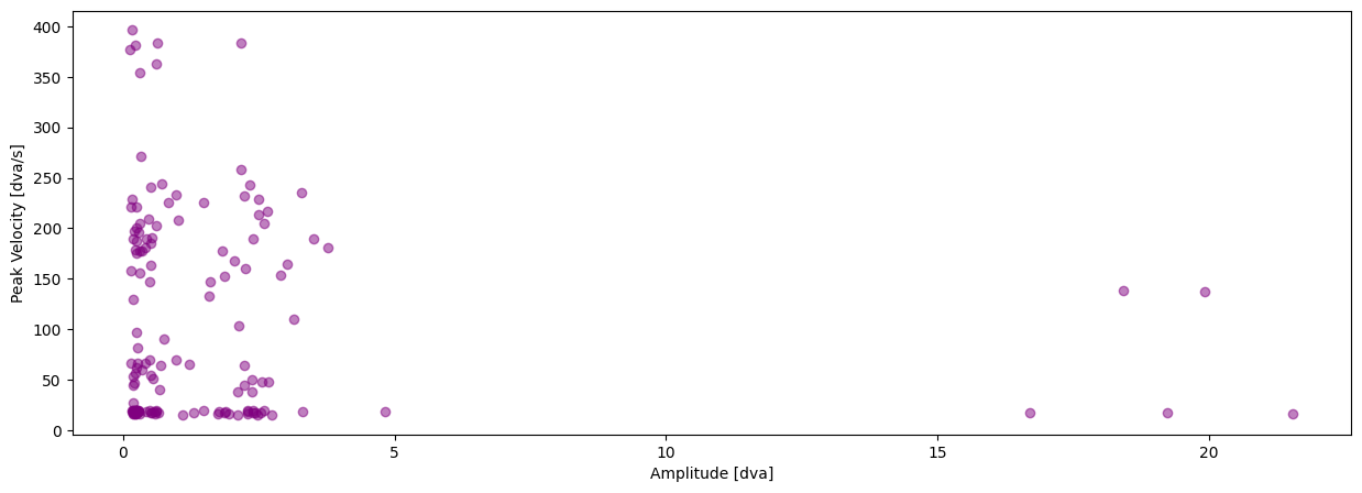
In this this tutorial we will plot the saccadic main sequence of our data.
[15]:
pm.plotting.main_sequence_plot(dataset.events[0])
Saving and loading your dataframes#
If we want to save interim results we can simply use the save() method like this:
[16]:
dataset.save()
100%|██████████| 2/2 [00:00<00:00, 1271.19it/s]
100%|██████████| 2/2 [00:00<00:00, 479.27it/s]
[16]:
<pymovements.dataset.dataset.Dataset at 0x7fa3e6ab57c0>
Let’s test this out by initializing a new PublicDataset object in the same directory and loading in the preprocessed gaze and event data.
This time we don’t need to download anything.
[17]:
preprocessed_dataset = pm.Dataset('ToyDataset', path='data/ToyDataset')

dataset.load(events=True, preprocessed=True, subset=subset)

display(dataset.gaze[0])
display(dataset.events[0])
100%|██████████| 2/2 [00:00<00:00, 1051.47it/s]
100%|██████████| 2/2 [00:00<00:00, 831.38it/s]
<pymovements.gaze.gaze_dataframe.GazeDataFrame at 0x7fa3e6206880>
<pymovements.events.events.EventDataFrame at 0x7fa3e6206e50>