Working with Raw Gaze Samples

Once gaze data have been loaded, they are available as time-ordered raw samples in gaze.samples.

The table below shows a basic example of raw gaze samples after import into pymovemnts. Each row corresponds to one time-ordered gaze sample and is stored in the samples attribute of the Gaze object. Timestamps are listed in the time column, and horizontal and vertical gaze positions in pixel coordinates can be found in the pixel column. Depending on the loader and input format, additional channels such as binocular coordinates or quality measures may also be present.

Show code cell source

Hide code cell source

import matplotlib.pyplot as plt

import pymovements as pm
from pymovements.gaze.experiment import Experiment

experiment = Experiment(
    screen_width_px=1280,
    screen_height_px=1024,
    screen_width_cm=38,
    screen_height_cm=30.2,
    distance_cm=68,
    origin='upper left',
    sampling_rate=250.0,
)

gaze = pm.gaze.from_csv(
    '../examples/gaze-toy-example.csv',
    experiment=experiment,
    time_column='time',
    pixel_columns=['x', 'y']
)

gaze.samples.head(5)

shape: (5, 2)

time	pixel
i64	list[f64]
0	[206.8, 152.4]
4	[207.0, 151.5]
8	[207.6, 151.9]
12	[207.6, 152.2]
16	[207.8, 151.6]

Inspecting Raw Samples with Plots

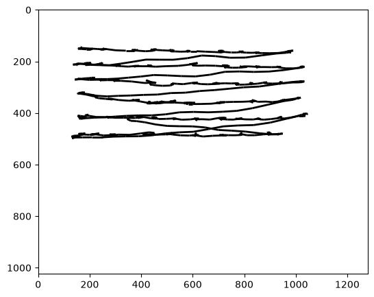
Visual inspection is an essential first step when working with newly loaded gaze data. Time-series plots help reveal signal loss, noise, blinks, sampling irregularities, or calibration problems before any preprocessing is applied. Using the traceplot() function, we can visualize raw gaze samples from a Gaze object. The plot shows the continuous trajectory of gaze positions across the stimulus, allowing inspection of spatial gaze behavior over time.

Show code cell source

Hide code cell source

pm.plotting.traceplot(gaze)
plt.show()

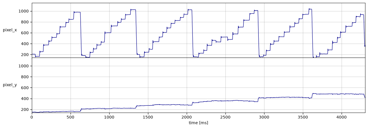
We can examine how each recorded signal changes over time by using the tsplot() function. It produces a time-series plot with one line per selected channel (e.g., horizontal and vertical gaze position). The x-axis represents time, as defined by the gaze sample timestamps. In this example, we plot the x and y channels.

Show code cell source

Hide code cell source

gaze_unnested = gaze.clone()
gaze_unnested.unnest('pixel')

pm.plotting.tsplot(
    gaze_unnested,
    xlabel='time [ms]',
    channels=['pixel_x', 'pixel_y'],
    share_y=False,
    line_color='darkblue',
    n_rows=2, n_cols=1,
    zero_centered_yaxis=False
)
plt.show()

Transforming Raw Samples

Raw pixel coordinates are tied to a specific screen setup and viewing distance. For meaningful interpretation and cross-experiment comparison, gaze samples are often transformed into alternative representations. These transformations operate directly on the raw samples and rely on the experimental metadata defined earlier.

pix2deg(): From Pixels to Degrees of Visual Angle

Eye trackers typically record gaze positions in screen pixels. While useful for display-based inspection, pixel units depend on screen size and viewing distance and are therefore not comparable across setups. The pix2deg() function converts pixel coordinates into degrees of visual angle (dva) using the experiment’s screen geometry and viewing distance.

Requirements:

• A pixel-based gaze column must be available (by default named “pixel”)

• An Experiment must be attached to the gaze data, because screen size and distance are needed for the conversion

gaze.pix2deg()
gaze

Gaze

• samples:
  DataFrame (3 columns, 4306 rows)
  shape: (4_306, 3)

  time	pixel	position
  i64	list[f64]	list[f64]
  0	[206.8, 152.4]	[-10.697598, -8.852399]
  4	[207.0, 151.5]	[-10.692768, -8.874233]
  8	[207.6, 151.9]	[-10.678275, -8.86453]
  12	[207.6, 152.2]	[-10.678275, -8.857252]
  16	[207.8, 151.6]	[-10.673444, -8.871807]
  …	…	…
  17204	[349.3, 420.0]	[-7.220662, -2.272553]
  17208	[362.7, 418.1]	[-6.89053, -2.319691]
  17212	[371.2, 419.0]	[-6.680877, -2.297363]
  17216	[365.9, 417.1]	[-6.811623, -2.3445]
  17220	[355.8, 413.8]	[-7.060582, -2.426362]

• events:
  Events
  Events

  • frame:
    DataFrame (4 columns, 0 rows)
    shape: (0, 4)

    name	onset	offset	duration
    str	i64	i64	i64

  • trial_columns:
    None
• metadata:
  dict (0 items)
• messages:
  None
• trial_columns:
  None
• experiment:
  Experiment
  Experiment

  • eyetracker:
    EyeTracker
    EyeTracker

    • left:
      None
    • model:
      None
    • mount:
      None
    • right:
      None
    • sampling_rate:
      250.0
    • vendor:
      None
    • version:
      None
  • screen:
    Screen
    Screen

    • distance_cm:
      68
    • height_cm:
      30.2
    • height_px:
      1024
    • origin:
      'upper left'
    • resolution:
      tuple (2 items)
      • 1280
      • 1024
    • size:
      tuple (2 items)
      • 38
      • 30.2
    • width_cm:
      38
    • width_px:
      1280
    • x_max_dva:
      15.599386487782953
    • x_min_dva:
      -15.599386487782953
    • y_max_dva:
      12.508044410882546
    • y_min_dva:
      -12.508044410882546

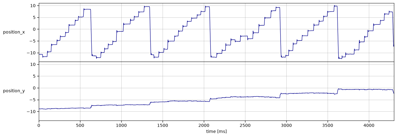
Unlike pixels, degrees of visual angle reflect the actual angular displacement of the eye relative to the observer’s viewpoint and are therefore comparable across different screen setups and viewing distances. In the plot below, the overall shape of the signal remains the same as in pixel space, since only the unit of measurement has changed. However, the scale of the y-axes differs, reflecting the conversion from screen-dependent coordinates to angular units.

Show code cell source

Hide code cell source

gaze_unnested = gaze.clone()
gaze_unnested.unnest('position')

pm.plotting.tsplot(
    gaze_unnested,
    xlabel='time [ms]',
    channels=['position_x', 'position_y'],
    share_y=False,
    line_color="darkblue",
    n_rows=2, n_cols=1,
    zero_centered_yaxis=False
)
plt.show()

pos2vel(): From Position to Velocity

Many eye-movement measures are derived not from position directly but from its temporal derivatives. Velocity is computed from changes in gaze position over time and is central to event detection algorithms for saccades and fixations. In pymovements, velocity is computed explicitly from position data with the pos2vel() function, using the sampling rate stored in the eye tracker definition.

gaze.pos2vel()
gaze

Gaze

• samples:
  DataFrame (4 columns, 4306 rows)
  shape: (4_306, 4)

  time	pixel	position	velocity
  i64	list[f64]	list[f64]	list[f64]
  0	[206.8, 152.4]	[-10.697598, -8.852399]	[null, null]
  4	[207.0, 151.5]	[-10.692768, -8.874233]	[null, null]
  8	[207.6, 151.9]	[-10.678275, -8.86453]	[1.610284, -0.101097]
  12	[207.6, 152.2]	[-10.678275, -8.857252]	[1.107104, -0.909672]
  16	[207.8, 151.6]	[-10.673444, -8.871807]	[0.6039, -1.617239]
  …	…	…	…
  17204	[349.3, 420.0]	[-7.220662, -2.272553]	[29.879682, -16.852411]
  17208	[362.7, 418.1]	[-6.89053, -2.319691]	[43.841686, -7.339814]
  17212	[371.2, 419.0]	[-6.680877, -2.297363]	[9.957777, -7.442396]
  17216	[365.9, 417.1]	[-6.811623, -2.3445]	[null, null]
  17220	[355.8, 413.8]	[-7.060582, -2.426362]	[null, null]

• events:
  Events
  Events

  • frame:
    DataFrame (4 columns, 0 rows)
    shape: (0, 4)

    name	onset	offset	duration
    str	i64	i64	i64

  • trial_columns:
    None
• metadata:
  dict (0 items)
• messages:
  None
• trial_columns:
  None
• experiment:
  Experiment
  Experiment

  • eyetracker:
    EyeTracker
    EyeTracker

    • left:
      None
    • model:
      None
    • mount:
      None
    • right:
      None
    • sampling_rate:
      250.0
    • vendor:
      None
    • version:
      None
  • screen:
    Screen
    Screen

    • distance_cm:
      68
    • height_cm:
      30.2
    • height_px:
      1024
    • origin:
      'upper left'
    • resolution:
      tuple (2 items)
      • 1280
      • 1024
    • size:
      tuple (2 items)
      • 38
      • 30.2
    • width_cm:
      38
    • width_px:
      1280
    • x_max_dva:
      15.599386487782953
    • x_min_dva:
      -15.599386487782953
    • y_max_dva:
      12.508044410882546
    • y_min_dva:
      -12.508044410882546

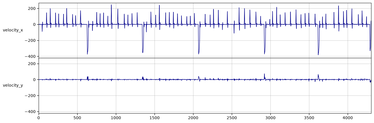
The following plot illustrates velocity, i.e. how quickly the eye moves at each time point. Periods of relative stability (low velocity) typically correspond to fixations, whereas sharp peaks in the signal indicate rapid eye movements such as saccades.

Show code cell source

Hide code cell source

gaze_unnested = gaze.clone()
gaze_unnested.unnest('velocity')

pm.plotting.tsplot(
    gaze_unnested,
    channels=['velocity_x', 'velocity_y'],
    share_y=False,
    line_color="darkblue",
    n_rows=2, n_cols=1,
    zero_centered_yaxis=False
)
plt.show()

For more information on these preprocessing steps, please see the Preprocessing Raw Gaze Data